Common valuation mistakes

General

Business valuations can be very complex. While forecasting many separate items, it is important to not lose sight of the bigger picture. The ValueModel is designed as a guidance for the analyst. Finally, you never again have to worry about incorrect formulas and calculation errors! However, there are still many mistakes that can be made, which is why we have this section. For support in double-checking your own inputs, we implemented ratios to measure proportions between certain important items. These ratios can be found in the “forecast” sheet below each section and are highlighted in dark green. The ratios can be compared to the firm’s ratio in the past to come to conclusions regarding your own input. – ’ ,

Using the wrong beta

Using the historical or too high/low beta: Before we start: High risk doesn’t mean high return. Furthermore, using the historical beta is likely to be incorrect. At A. Stotz Investment Research, we recently tested what happens to beta over time among an average of 10,000 stocks around the world. The findings imply that when you value a stock with a historically low beta, a good beta estimate would be about 0.7x and for a high beta stock about 1.1x. When a stock historically has had a neutral beta of 1x or you are forced to make a guess about beta without any information, your safest choice would be to set beta to 1x. For exactly this reason we recommend a beta-range of 0.75 to 1.25. A. Stotz framework suggest choosing 1.25 for historical betas of 1.15 and higher, choosing 1 for historical betas between 0.85-1.15 and choosing 0.75 for all historical betas below 0.85.

Using the wrong risk-free rate

Using historic or short-term risk-free rate: To use the historic average of the risk-free rate is incorrect. The risk-free rate is the rate that you can currently obtain by buying long-term government bonds. This means using bonds with similar duration to your cash flows.

Inconsistent estimates: To build your reputation and become a respected analyst, you have to be consistent with your estimates. This means having the same assumption for the risk-free rate for all valuations within the same market. It would not make sense to apply different risk-free rates to different companies within the same market.

Reconciling the company’s cost of debt with the risk-free rate: When choosing the risk-free rate, it is important to remember that the risk-free rate is “embedded” in all interest rates in that country. For domestic investors, the risk-free rate should be the lowest rate in that country because it is supported by the full faith and credit of that country’s government. In other words, they can always print more money to pay the interest. So if the risk-free rate is 4% in a country the rate that a company would pay would be higher than that by maybe 1-5% depending on the credit risk of that company.

When forecasting a company’s interest rate it pays on debt it is important to reconcile this with your assumption on the risk-free rate. For example, let’s say you were valuing a company in Hong Kong, where the risk-free rate has been about 2% over the prior years, compared to valuing a company in Indonesia where the risk-free rate over the same time was 9%. You would then want to imagine that the rate that the company pays is some premium over this risk-free rate. Start by looking at the company’s interest rate in the past and consider that relative to the past risk-free rate. Then look forward and decide whether the gap between the rates would widen (if the company’s debt is becoming more risky, or corporate debt in general is becoming more risky) or reduce.

Going back to our Hong Kong case, imagine a risk-free rate of 2% over the last 3 years and that the company paid 6% over that time period, a 4% premium. If you forecast that risk-free rate will rise to 3% going forward and you assume that the riskiness of the company will stay the same, then in theory the interest paid by the company would be 7%. Of course, there is not perfect answer to this dilemma, however, thinking about this carefully will prevent you from making an obviously inconsistent assumption.

Fade period calculations and assumptions

To make consistent assumptions about the firm you are forecasting, it is critical to understand how the ValueModel is calculating cash flows and what exactly will be faded.

Change in invested capital: Depreciation, CAPEX and the change in working capital are not forecasted in detail for the fade period. As a substitute, we calculate invested capital growth during the discrete period instead and fade this growth rate down to your estimated growth rate.

ROIC: As firms get into a mature state, their profitability usually decreases to some extent. Only the most profitable firms such as Microsoft have managed to achieve excessive returns over a long period. The second step we are taking during the fade period is to decrease linearly ROIC to the level of WACC. However, there is an additional option to fade ROIC to WACC + a 20% premium or discount for extremely high/low profitability firms.

Through our assumptions for ROIC and invested capital, we come up with a smooth transition of cash flows from the discrete to the fade and the terminal period.

Using the wrong market risk premium

Inconsistent estimates: To build a reputation as a respected analyst, you have to be consistent with your estimates. This means having the same assumption for the market risk premium for all valuations within the same market. It would not make sense to apply different market risk premiums to different companies within the same market.

Using historical market risk premium: Similar as for the risk-free rate and the beta, using historical extrapolation as inputs to determine the market risk premium should be reduced. Instead, we should focus on a more forward-looking analysis. Opinions about expected returns are usually based on historical average returns, financial and behavioral theories and future market indicators. To come up with a reasonable risk premium estimate, we have to take all those factors into consideration. Using historical data is difficult because it depends on the timeframe you are looking. A short time window might lead to biased data that includes one-offs that are unlikely to be repeated in the future. Long time windows reduce bias, but might include structural changes that do not apply to current standards. Furthermore, they include cyclical variations of expected returns and survivorship bias. Studies have shown that high-return periods are often followed by low-return periods and vice versa.

Expected market risk premium: A common way to determine the expected market risk premium is to survey a big number of financial academics and professionals and average their estimates for future market risk premium. While this approach clearly has benefits, it is necessary to point out that human beings seldom share homogeneous beliefs, and this results in volatile outcomes. Furthermore, humans are prone to bias and to underestimating the cyclical variations of expected returns.

Implied equity premium: This view on market risk premium is based on the assumption that markets price stocks correctly on average. We are able to estimate the expected market returns and can subtract the risk-free rate in order to arrive at the implied market risk premium. To estimate the implied equity premium, dividends or earnings yield are commonly used. An advantage of this estimation is that it captures recent market developments while a disadvantage is that it is extremely sensitive to growth rate assumptions.

Here is some general advice we want to share with you in making better estimates: 1. Collect risk premiums from various sources. 2. Research finds the least predictability in the historical risk premium. 3. Which premium to choose generally depends on the purpose of your analysis, your beliefs about the market, and the importance of predictive power to you.

Include our market risk premium research from Become a Better Investor

Firms that are listed abroad and multinational companies: For some firms, it can be very difficult to decide which discount rate to use. Some businesses are located (and generating revenues) in one country (such as China), but are listed in another country (for example, Singapore). In this case, should we use the equity premium of  China or Singapore? Since the discount rate reflects the riskiness of cash flows, we should always base our estimates on the market of which the revenues are derived from – in this case, China. Some people even go so far to say that for multinational companies one should have separate estimates for each and weight them to arrive at the final figure. However, as weights of revenue streams change over the lifetime of a business, this procedure has a huge downside to it as well.

Optimism bias

We at A.Stotz Investment Research have been asking the following question: Are financial analysts’ earnings forecasts accurate?

Different to the many other research papers on this topic, we scaled the analysts’ errors by earnings and not by price. Scaling by earnings has the benefit of making your results comparable as the share price could be wildly swinging per time and from stock to stock.

Conventional method: (Forecast earnings – Actual earnings) / Share price = SFE
Method used by A.Stotz: (Forecast earnings – Actual earnings) / |Actual earnings| = SFE

The results show that analysts were 25% optimistically wrong over the 12-year period used. During the best years, they were only wrong by 10%. In 2008, the worst year, when earnings collapsed, they were wrong by 55%. That’s interesting right there. At that point, basically, the analysts probably didn’t move much. Instead, what happened was that earnings collapsed. What we found as well is that analysts were never pessimistically wrong.

Looking at emerging markets, we found that the analysts’ error was 35%. Emerging markets analysts had been much more optimistically wrong, especially from the period of 2010 to 2014.

Imbalance between assets and source of funding

Building up too much cash and not growing fixed assets fast enough: If a company is building up cash it is usually a good sign. Liquidity ratios improve and the company has fewer difficulties covering their short-term liabilities. However, when using financial models, this can also happen by accident. Let’s say you are valuing a high growth company: the company had a rough patch in the recent past but the completion of a very profitable plant is imminent and you expect the earnings to increase massively. Some analysts would accelerate the revenue growth rapidly but wouldn’t increase the asset growth in an appropriate intensity. These receipts are then booked as cash. The result is that your forecast is suggesting that the company is building up huge amounts of cash when in fact it might be an unrealistic assumption as a strongly growing company would probably invest more heavily to generate further growth. Another consequence of this mistake would be that in some cases net fixed assets will be decreasing in your forecast, which is rarely the case in reality (we suggest at least 3% in net fixed asset growth).

If you have grown your assets fast enough and there is still too much cash, it would be reasonable to assume the company is going to pay them out as dividends rather than holding the cash if they haven’t done so in the past. Therefore, it is of importance to always keep an eye on the “Cash & short-term investment/sales” ratio.

Override cash forecast when no ST-debt: By using the ValueModel you might be curious why in some cases the “Cash & short-term investment/sales”-ratio does not influence the actual number for “Cash & short-term investments”. The reason for this is that your input is causing short-term debt to be negative which is not possible. As a result of that, the model will build up cash and overwrite your suggested input. “Cash & short-term investments” and “Overdrafts & short-term debt” are used to balance out assets and liabilities, so in that way you can think of them as a plug.

Too much ST-debt when growing assets too fast: “Cash & short-term investments” and “Overdrafts & short term debt” are used to balance out assets and liabilities, so in that way you can think of them as a plug. Whenever “Overdrafts & short-term debt” gets unrealistically high, the problem is the discrepancy between assets and the source of funding. It can be avoided by growing liabilities faster (Long-term borrowing growth, Other long-term liability growth, Other current liabilities/sales). Once you finance your capital spending properly with those items, short-term debt will be reduced automatically.

Relationships between items

Many analysts are unsure about the relationship between certain items that they are forecasting.

Depreciation and Capex: As a rough estimate, CAPEX should be around 150% of the amount of depreciation. CAPEX usually consists of maintenance CAPEX, which is the investment amount needed to maintain the current fixed assets to generate revenue, and the growth CAPEX. The maintenance CAPEX should be roughly the same amount as depreciation – while machinery depreciates over time, the firm will replace such machinery with new items to maintain its business. However, if the company wants to grow, as they usually do, they need to invest a substantial amount additionally in the maintenance CAPEX. This is called growth CAPEX and that is the reason why CAPEX must be higher than depreciation.

Huge jumps in free cash flow growth

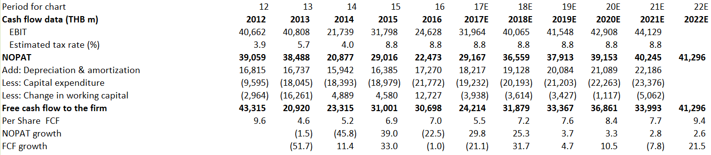
Huge changes in cash flow within two consecutive years are unrealistic if they are not justified. However, under some conditions there can be big gaps between the cash flows of two consecutive years without immediate detection by the analyst. This happens to be the case for the transition between the actual forecasted period (discrete period) and the fade period. As some items are not explicitly forecasted beyond the discrete period it increases chances for unsmoothly forecasted cash flows. These gaps can be easily spotted by examining the free cash flow growth (FCF growth) in the “DiscountVal” sheet. A high FCF growth in the first year of the fade period might overvalue the firm.

The table below displays such a case. As depreciation & amortization, CAPEX and the change in working capital are not projected into the fade period in 2022, free cash flow to the firm increases 21.5%.

Fixed asset growth is negative or close to zero

As a rule of thumb: Fixed asset growth should roughly match revenue growth. If you don’t expect a revenue growth of 0%, fixed asset growth should not be zero as well. In all other cases we would recommend that you not grow fixed assets below 3%. An easy way to check your assumptions is to have a look at the asset turnover ratio in the forecast sheet under “Forecast variables: Assets” – “Revenue per >currency< of assets”.

Forecasting the change in working capital

Sometimes it can be difficult to forecast the change in working capital of a company. Therefore it is necessary to focus on the main idea of working capital. A question you need to ask yourself is whether the company is spending in advance of its growth. If it is, the change in working capital should be negative as a percent of the change in revenue. A typical example would be a retailer: it has to buy inventory before it sells it to its customers, so it is going to spend money on working capital before it can actually realize sales from spending that working capital. As a result it needs more cash to grow as its sales grow. On the other hand, there are companies that have the opposite situation where they actually get money as a result of their growth. A classic example is any subscription company where it gets money from customers in advance before it delivers the service. If that is the case, the change in working capital will be positive as a percent of the change in revenue. As a company’s revenue grows, it gets additional cash from those business units (collection of cash from customers up front).

To forecast the change in working capital you can use several approaches:

1. Grow the last change in WC at the expected growth rate of earnings. 2. Measure WC as a percent of Revenues and use that ratio to forecast. 3. Measure WC as a percent of Revenues over a historic period and use that ratio to forecast. 4. Forecast based on the industry’s average working capital as a percentage of revenues.

Terminal value assumptions

The terminal growth rate is used to determine the value of a company within the terminal period. It is the stable growth rate the firm can sustain in perpetuity and it can range between 0% and 5% in the ValueModel. The terminal growth rate should never exceed the growth rate of the economy. Theoretically, the stable growth rate could also be negative but this would mean that the analyst is assuming the firm to disappear over time. A simple proxy for the growth of the economy can be the risk-free rate.

The formulas to arrive at the terminal multipliers in the model are:

For DCF valuation:  Terminal multiplier = 1/(WACC-g)

For DDM valuation: Terminal multiplier = 1/(k-g)

Forecasting an increase in equity

There are some scenarios in which an analyst could justify the forecast of an increase in equity, however, we generally advise against it, unless the company already announced it would do so but had yet to execute it. There are three reasons for this: 1. Owners usually don’t want to increase equity because it may cause dilution. 2. We don’t have any indication that the company needs more capital. For all we know the company could slow down its growth. 3. We use overdrafts and short-term loans as a plug to make the balance sheet balanced. If assets grow fast but long-term debt does not, short-term debt will fill out the difference. Whether it is reasonable to increase long-term debt has to be decided based upon the company’s financing history.

Forecasting capital expenditures

There are two types of capital expenditure (CAPEX). One of them is the maintenance CAPEX which is an investment that is required to keep the business running at its status quo. Among other things, this includes new computers to replace old technology, therefore it will not grow the business or attract new customers. As a rough estimate of the maintenance CAPEX, you could use depreciation and amortization. To fund different projects, increase the capacity of the business or attract new customers, the company has to invest in its growth CAPEX. Forecasting capital expenditures of a company can be challenging. There is no rule of thumb to be used in every scenario, however, we collected a few rules to guide you:

1. If the company has only a small amount of depreciation, it can indicate that it is operating old assets. In this case, it would be reasonable to forecast higher CAPEX, which includes the renewal of assets.

2. Depreciation can never be higher than CAPEX in perpetuity.

3. Some analysts use a CAPEX of zero because they do not have specific information. This is incorrect since a CAPEX of zero highly overvalues the company as the free cash flows will be higher than they should be (as CAPEX is not subtracted from NOPAT).

Using multiples to value a company

When using multiples to value a company you are basically taking a known item, such as earnings or book value and convert it to a price. It is based upon the law of one price – that is that similar assets should be sold at similar prices.  This has the advantage that it is easy to use and is based on actual market transactions. However, there are also significant disadvantages that are associated with valuation using multiples. Here are some of the reasons we do not recommend multiple valuation:

1. It is difficult to find comparable companies for a timely comparison.

2. The underlying assumption that prices paid for comparable companies were realistic.

3. The range of multiples for companies operating in the same industry can be huge.

Recency bias

Recency bias is a cognitive bias that causes people to deviate from rationality and good judgment. Such a bias causes people to focus on what happened recently and lose sight of the bigger picture. When it comes to forecasting, it means that the analyst is more influenced by the last – let’s say – 1-2 years than by the periods prior to that. In trading, this can mean that you get reluctant to trade if you have good trading stats and lose a couple of times in a row. It can also lead to a frequent change in strategy.

Goodwill

Goodwill is an intangible asset such as intellectual property or brand names. As intangible assets are not physical, they are difficult to value. Goodwill projects the premium paid by the purchasing party on top of the fair market value of an asset which can be attributed to intangibles, such as reputation, brand or human capital.

Without a write-down of goodwill, it will be captured forward in the balance sheet.

Forex/revaluation/other

Coming soon..

Debt

Debt levels

A mistake analysts make frequently is to forecast a high amount of debt in the fade and terminal period leading to an overvaluation of both FCFE and FCFF. If we focus on FCFF, high amounts of debt can lead to having a very low discount rate (WACC), hence the high value within the terminal period. Our research shows that anything equal to or over 55% of debt of the capital structure is considered very high as it would be very rare for a company to finance itself forever with this high debt level.

This basically means the bankers are putting more money into the company than the equity owners. It may be possible for short periods of time (usually when the company is distressed) but is highly unlikely over long periods. Our research shows that debt should be around 30% of the capital structure for the fade and terminal period. It could be higher, but not by much. This will help to reduce and stabilize the value of the terminal period in the FCFF.

Debt covenants

Imagine you lent money to an unemployed friend who was in a desperate financial situation. Then you see he moved to a more expensive apartment, bought a fancy car, and you see him in an expensive restaurant. Do you think you will be repaid? Unlikely.

Now imagine that you lent him money on the condition that he did not spend ANY of his money on extravagant things until you were paid back. If he signed that agreement then you would have set some “debt covenants” that he must follow.

The same thing happens when a business borrows. The company and its creditors will agree to limits within which a company will operate. This is a lender’s way of preventing the management from running the business in such a way that it becomes unlikely that the business will have the capacity to repay the lender.

Here are general some general covenants, I have stated them all in the negative (do not), though they can be stated in the positive (do).

Do not borrow too much more. One covenant could be to maintain a net debt-to-equity ratio below a certain level. This prevents the company from borrowing more money from others.

Do not remove capital from the business. One covenant could be on the amount of dividends allowed to be paid out to shareholders.

Do not let your business profitability fall below some point. One covenant in this area is interest cover or the times interest is earned. Which is some measure of profit (EBIT, EBITDA, etc.) divided by the regular interest payment required. This prevents the company from paying itself big bonuses, running up costs, or neglecting the core profitability of the business.

Do not manage your working capital in such a way that your cash flow deteriorates. One covenant example could be that the company must maintain 35 or less days accounts receivable outstanding.

Do not damage the future growth opportunities of the business. One example of this is to sell a core asset without the approval of lenders. A covenant in this area could be a restriction on selling certain assets.

Do not do strange things. Do not change auditors, do not be late on financial reporting, do not change significant accounting policies.

Sometimes debt covenants are referred to as positive (things to do, such as maintain EBITDA margin above xx%) or negative (do not allow net debt-to-equity rise above xx).

If you break these covenants, you could be forced to sell asset or take other drastic action to allow the bank to recover its money. Another action is that you may be required to raise new equity capital.

So in your case, a company usually maintains a steady net debt-to-equity, but occasionally that could shoot up, like in the case of borrowing for an acquisition.

In your case you forecast that long-term debt will fall, that is unlikely. Here is why…

When forecasting long-term debt remember that this can be a “lumpy” item. What that means is that a company could go from zero long-term debt to one hundred million in one period. That is the period that the company either borrowed from the bank or issued long-term bonds. You can usually assume that the company will keep that long-term debt for 3-10 years. It is rare that that amount will go down immediately. In other words, long term borrowing is a long-term capital management decision. For example, let’s say that short-term interest rates had been super low so the management of a company would be happy to borrow short-term money. However, ultimately a company wants a stable supply of funding, so when the management thinks that short-term interest rates are going to rise they may switch that borrowing to long-term borrowing. One other common situation is if the company has an immediate opportunity to buy some assets (another company, machinery, etc.), they may get a short-term “bridge” loan to finance such a purchase. This loan bridges the time gap necessary to do all the paperwork to borrow long-term funding. Then after the purchase is made they replace the bridge loan with a long-term long. It could be completely different companies that lend the bridge loan money, a company that has a higher risk profile.

Seasonality in Revenue Forecast

A common valuation mistake analysts do a lot of times is not considering seasonality in revenue forecast. Financial data in companies is usually announced on a quarterly basis. Companies with a certain type of business have high and low revenue quarter. For example, an air-conditioner company’s high revenue quarter will be during summer time. The problem occurs when analysts use these high revenue quarter and annualize them to create a forecast.

In other words, if you have to forecast the current year’s revenue growth for the company and the company’s first quarter is seasonal high for the revenue, you may probably make a mistake multiply this revenue number times four and forecast the revenue for the year. Unless the company has very low seasonality, be careful or try to avoid the quarter-on-quarter (QoQ) comparisons.

Two possible solutions to this problems are:

1.  Consider year-on-year (YoY) growth by comparing the first quarter this year against the first quarter last year.
2.  Calculate a rolling four-quarter revenue number and compare that to a rolling four quarter number from the prior period. To do this you would sum up the prior four quarters, starting with the most recent and then do the same for the prior period.

Unreasonably high level of Return on Equity (ROE)

This is a common valuation mistake made by analysts of forecasting ROE extremely high. This mistake can be caused by a few possible errors:

1.  Net profit margin being too high
2.  Company is expected to borrow a lot which can cause the profits earned to be very high on the same level of equity
3.  A too high or significantly rising dividend payout ratio