Valuation Master Class forecasting guidance

The ValueModel is a three-stage model can be applied to cover three phases of a company’s growth life cycle (high growth, low growth, smooth transition between the two phases).

The first of the three stages is the discrete period that covers the first 5 years of forecast in which all items are forecasted precisely based on your assumptions, the terminal period which uses a low growth rate that can be sustained into perpetuity and derives the value for future years, and the fade period which connects the discrete period with the terminal period by fading profitability, growth and others.

For this forecasting guidance, I will focus on the forecast and discountval sheet and share my thoughts on how to establish solid assumptions. The forecast section is divided into three major categories: P&L, balance sheet and cash flow statement.

Important: Always look at the actual numbers (instead of just the ratio or growth rate) when applying your assumptions. The forecast variables usually include growth rates or ratios (e.g. revenue growth, other current assets/sales etc.) which can be extremely volatile or misleading. What matters most is not that the growth rates are in line with historical averages but that the actual numbers are as wished.

Note: Sometimes I name the forecast variable, sometimes the actual item from P&L or BS. This is based on which number I finally check when doing my forecast. In some cases, it does not make sense to look at very volatile growth numbers, but instead look at actual numbers and the CAGR. I strongly suggest you use the CAGR button in the ValueModel (Ribbon “ASIR FIN MODEL”). Just mark the relevant cells and click the button to receive the compound annual growth rate.

When doing valuation, it is always important to look at the bigger picture. Please keep in mind that there are only four ways to increase value: increasing revenue, reducing cost, reducing the investment amount and reducing risk.

If you have absolutely no idea how to forecast a certain item, our common-size P&L and balance sheet analysis by industry can give you an indication: https://slimwiki.com/a-stotz-investment-research/sector-specific-issues

FORECAST SHEET Profit and loss

1. Revenue – is also referred as Sales. We need to find out some factors from different sources (analyst report, news, industry growth rates etc.) that would affect the revenue. Using analyst reports as revenue guidance can be misleading. Several studies have found that analyst are usually optimistically wrong about the company’s future revenues (globally by 25%, in emerging markets by 35%). Therefore, it is reasonable to use these forecasts as an upper bound. Industry growth rates can give a good guidance on future revenue growth when considering the firms competitive power and market share. Sales is heavily influenced by the success of existing products, new product development, product gaps and the products in comparison to competitor’s products. A porter five forces analysis can help to provide a sound judgement of future sales growth. Generally, the revenue tends to increase in the future since the company wants to make profit and this is done by increasing revenue or profitability. Additionally, to the approach mentioned above, the historical CAGR can give an indication on future revenue growth. Please note that it gets tougher to maintain the same revenue growth numbers as the company gets bigger. By that I mean it is easier to grow by 10% when your sales is THB 10.000 compared to THB 100.000. Therefore, the forthgoing CAGR should in most cases be a bit lower than the historical CAGR. Be aware of, and make sure to deal with seasonality.

2. Gross profit margin – Often analysts will forecast the future GPM and justify their prediction with facts – we can use this information for our forecast. For example, if the company introduces a new product with higher margin or oil prices are expected to decrease soon. This is likely to increase the GPM in the near future.  Another approach is to use 1. the average GPM from the past years (only if the volatility is rather low) or 2. An extension of the current trend in numbers (if the GPM kept increasing in the past 5 consecutive years it might make sense to continue this trend after checking for reasons).

3. SG&A/sales – Refers to costs for a company in comparison to sales. Higher revenue does not necessarily mean that SG&A/sales is going to increase. It is possible that a company is able to cut the cost through economies of scale. Cost cutting programs are often announced by the company itself or researched by other analysts – this information should influence our forecast in a reasonable way (firms will always say that they will increase GPM or cut costs, but it is your job to judge whether their effort will be successful or not, based on their reasoning). Another approach is to use 1. the average SG&A/sales from the past five years (only if the volatility is rather low) or 2. an extension of the current trend in numbers (if SG&A/sales was increasing in the past 5 consecutive years it might make sense to continue this trend after researching the reasons).

 

4. All “Other…” – items (e.g. Other operating (exp.)/income, Other non-operating (exp.)/income, Other current assets/liabilities, Other long-term assets/liabilities) includes several different items. It is always important to check which of these items is significant. Based on this fact you can make the decision on how much time to spent to forecast it in detail. If one of those items is very substantial, it might make sense to check the firm’s financial statement if there is huge fluctuation in the numbers, in cases where the number is rather small it might be enough to use the CAGR for your forward forecast. Generally, these items grow as the business grows. Rule of thumb: Other long-term assets/liabilities growth should be equal or lower than total assets/liabilities growth.

5. Interest expenses – It is based on the government bond yield of each country. We usually forecast the interest expenses based on past data. It seems that interest expenses tend to stay the same or increase a bit since the historic interest rates are on an all-time low currently and are expected to increase in the future. For evidence see: http://static4.businessinsider.com/image/54ea4a8869bedd1b3d230906-1006-694/chart-86.png

6. Income tax – Google “(Country) corporate tax rate” and you will find the income tax for each country. Each country has a different effective tax rate. Furthermore, the tax in the historic numbers does not necessarily have to be the current actual corporate tax rate as some firms might get tax benefits for some time. If you are unsure it is better to take the more conservative tax rate that does not include tax benefits.

7. P&L equity income/BS LT investments –  Income generated from investments in other companies where the firm owns more than 20% but less than 50% of the shares thus it does not possess controlling power over the associate. If the firm owns more than 50% of the company, the company is considered a subsidiary and both firms financial statements are consolidated (see minority interest). Use the average actual number or the historic CAGR to forecast this item if the item is not substantial. However, if it is substantial, it makes sense to research in detail how much is contributed by each associate to have a more precise forecast.

8. Minority interest is registered for parent firms that own more than 50%, but less than 100% of the shares in another firm. This results in a consolidation of their financial statements, but since not 100% of the subsidiaries shares are owned by the parent company, not 100% of the profits are distributed to it. Minority interest is the amount of profit that does not belong to the parent company.

 

9. Foreign exchange gain/(loss) – we barely forecast a loss or gain due to foreign exchange rate since the exchange rate in the future is unpredictable. Since we can’t predict currency movements in the future, we usually don’t forecast this item (just keep it zero). One exception would be if we have 3 quarters of data indicating a big gain or loss – in this case we would forecast it for the current year.

 

10. Exceptional item – Some factor that cannot be predicted. This item usually includes accidents like floods or fire in the factory, earthquakes etc. It is unpredictable and unlikely to happen again in the near future. Therefore, we usually do not forecast it. There might be an exception if the gains or losses occur on a consistent basis with low volatility.

 

Assets

1. Cash & short-term investment/sales – It is the amount of cash that the company holds in relation to their revenue as well as short-term investments that are considered very liquid and can quickly be turned into cash. Generally, the company does not want to hold a lot of cash. They would use excess money rather to invest or expand their company. For asset-heavy companies (like materials) cash levels might be higher than for asset-light companies (like information technology). The reason for firms to keep cash is as a buffer or safety net. In case something unforeseen happens, the firm needs immediate liquidity to deal with the issue to avoid financial distress costs. Keep cash levels with the recent historic number or follow the recent trend. In the short-term, cash levels can decrease when the firm takes on expensive projects. On the other side, an increase in cash levels could also mean that the firm has limited investment opportunities. By using the ValueModel you might be curious why in some cases the “Cash & short-term investment/sales”-ratio does not influence the actual number for “Cash & short-term investments”. The reason for this is that your input is causing short-term debt to be negative which is not possible. As a result of that, the model will build up cash and overwrite your suggested input. “Cash & short-term investments” and “Overdrafts & short-term debt” are used to balance out assets and liabilities, so in that way you can think of them as a plug.

2. Receivables collection period – approximate amount of days that it takes for a company to receive outstanding payments. We use the historical average or trend to forecast it. Changes in the company’s credit policy influence the forecast. If accounts receivable grow much faster than sales, it can be an indication of cooked books.

 

3. Inventory conversion period – approximate amount of days that the inventory takes from being produced to being sold – Raw materials and supplies, products that are in production, and finished goods. We use the historical average or trend to forecast it.

4. Long-term investments – The company’s investments that tend to be held for more than a year, e.g. investments in stocks (can be ownership in associates), bonds, real estate. If we do not have specific information about upcoming partnerships or investments, we use the historical average or trend to forecast it.

 

5. Gross fixed assets – Gross fixed asset growth is directly influencing CAPEX. Capex is the total funds to invest in new projects, buy or upgrade physical assets, e.g. property, plants, and equipment. If your company is USPS, all transportation vehicles that use to deliver mails will be counted in CAPEX. Maintenance CAPEX is the minimum and should be roughly the same as depreciation. CAPEX is always higher than the depreciation since it consists of maintenance CAPEX (should roughly be the same as the depreciation amount as it is used to maintain the current business) and growth CAPEX (actual growth). CAPEX usually increases overtime since the company pushes growth and expansion. In a normal case, we set CAPEX to around 150% of depreciation and higher/lower if the firm’s growth profile deviates from “normal”. A general rule for net fixed assets growth is that it cannot be lower than 3% unless there is no revenue growth and even then, it has to be justified by the analyst since it is highly unlikely. Net fixed asset growth should roughly match revenue growth, because it’s unrealistic that assets will grow faster than the company’s revenue (in most cases).

6. Depreciation –  Average numbers of years assets are depreciated over. Look at the trend of depreciation (usually depreciation increase overtime as your assets base increases). Huge changes in the life of an asset might be an indication for a company to cover up bad accounting results. A general rule to follow is that CAPEX should roughly be around 150% of the amount of depreciation for a firm with average growth. Depreciation itself can be forecasted using the historical average or trend.

7. Asset under construction – Funds that are currently used for Tangible assets that are not yet finished, e.g. buildings or equipment that takes a longer time to build. Assuming a firm would build a new factory over the next 2 years with costs of 500 million and we do not have the exact distribution of costs over those 2 years: Year 1 AUC would be THB 250 million; Year 2 AUC would be THB 500 million and year 3 would be THB 0 AUC since the project is finished and start to depreciate. If you have specific project information you can build them into this figure, however as this can result in a highly volatile CAPEX, you should rather conservatively treat this item if you do not have precise information.

 

8. Increase/(Decrease) in intangible assets – A change of intangible asset value from the previous year which is difficult to predict. An intangible asset is an asset that is not physical in nature, including intellectual property, patents, trademarks, and copyrights. I would predict a forecast based on CAGR in the case of persistent increases in the past.

9.  Increase/(Decrease) in goodwill –  Sum of changes in goodwill during the current year. Goodwill is the additional price a firm pays when purchasing another firm on top of the fair value

 

Liabilities

1. Overdrafts & short-term debt – An account made up of any debt incurred by a company that is due within one year. It can only be adjusted in the model indirectly. “Cash & short-term investments” and “Overdrafts & short-term debt” are used to balance out assets and liabilities, so in that way you can think of them as a plug. Whenever “Overdrafts & short-term debt” gets unrealistically high, the problem is the discrepancy between assets and the source of funding. It can be avoided by growing liabilities faster (Long-term borrowing growth, Other long-term liability growth, Other current liabilities/sales). Once you finance your capital spending properly with those items, short-term debt will be reduced automatically.
2. Current portion of long-term debt – Total amount of long-term debt that is due within one year. Use the average of actual number to forecast.
3. Payables deferral period –  Average number of days it takes for the company to pay its suppliers when the company has purchased on credit. We use the historical average or trend to forecast it.
4. Increase/(Dec) in long-term debt– Increase/decrease amount in long-term debt during the year. For example: Increase can be a new bank loan or a new bond issuance. Decrease can be repayment of a bank loan. Look at the actual number to forecast and elaborate on the firm’s story and activities. If the firm just invested in major projects, long-term debt might increase up to the forecast period. However, this trend does not mean that it will continue forthgoing. Usually firms pay off some of their debt before engaging in new major projects.

Other important input (forecast sheet)

1. Change in working capital – Sometimes it can be difficult to forecast the change in working capital of a company. Therefore, it is necessary to focus on the main idea of working capital. A question you need to ask yourself is whether the company is spending in advance of its growth. If it is, the change in working capital should be negative as a percent of the change in revenue. A typical example would be a retailer: it has to buy inventory before it sells it to its customers, so it is going to spend money on working capital before it can actually realize sales from spending that working capital. As a result, it needs more cash to grow as its sales grow. On the other hand, there are companies that have the opposite situation where they actually get money as a result of their growth. A classic example is any subscription company where it gets money from customers in advance before it delivers the service. If that is the case, the change in working capital will be positive as a percent of the change in revenue. As a company’s revenue grows, it gets additional cash from those business units (collection of cash from customers up front). To forecast the change in working capital you can use several approaches: 1. Grow the last change in WC at the expected growth rate of earnings. 2. Measure WC as a percent of Revenues and use that ratio to forecast. 3. Measure WC as a percent of Revenues over a historic period and use that ratio to forecast. 4. Forecast based on the industry’s average working capital as a percentage of revenues.

2. Dividends – It is the only way to get money out of a company. Usually companies aim to increase their dividend payout as they grow. Research shows that firms (especially banks) are very reluctant to lowering their dividend payout ratio as this gives a negative signal to the market. Therefore, we usually forecast the same level or an increase based on the firm’s financial situation.

DISCOUNT VALUATION SHEET Cost of capital assumptions

 

1. Market – use the country that firm is located or where it generates most of it’s revenues.

2. Market risk-free rate – Take the 10-year government bond yield as proxy for the risk-free rate.

3. Market equity risk premium – There are three possibilities to choose from: Historic equity risk premium, expected equity risk premium and implied equity risk premium. However, as we forecast into the future, we want to use the figure that has the best predictive value. Historical equity risk premium is easy to calculate, equal for all investors but has little predictive power. Expected equity risk premium can be in the form of a survey. There are studies that ask a huge number of financial firms and academics about their risk premium predictions for the future and summarizes the results. The problem with this approach is that investors don’t share homogeneous predictions and the estimates can be biased. Research found the most predictive power within the implied equity risk premium. Usually dividends or earnings yield is used to calculate the IERP. This method assumes that market prices are correctly priced and captures recent market developments but it is very sensitive to growth assumptions. You can google to find estimates for the implied equity risk premium for each country.

–

4. Company beta – A beta of less than 1 means that the security is theoretically less volatile than the market. A beta of greater than 1 indicates that the security’s price is theoretically more volatile than the market. When a stock historically has had a neutral beta of 1x or you are forced to make a guess about beta without any information, your safest choice would be to set beta to 1x. For exactly this reason we recommend a beta-range of 0.75 to 1.25. A. Stotz framework suggest choosing 1.25 for historical betas of 1.15 and higher, choosing 1 for historical betas between 0.85-1.15 and choosing 0.75 for all historical betas below 0.85. Take the historic figure to come up with your beta estimate within our framework. Don’t forget, that beta is forecasted to infinity.

5. Cost of debt – This is basically the same item as interest expense for the fade and terminal period. As rates are currently on an all-time low, we use historical numbers and increase them slightly before we use it as input.

–

6. Average tax rate – Find corporate tax of the country the firm is operating in (see corporate tax in P&L). While for the discrete period there still might be tax benefits, for the fade and terminal period we usually forecast the full corporate tax rate.

7. Debt as a % of total capital – A mistake analysts make frequently is to forecast a high amount of debt in the fade and terminal period leading to an overvaluation of both FCFE and FCFF. If we focus on FCFF, high amounts of debt can lead to having a very low discount rate (WACC), hence the high value within the terminal period. Our study on 500 of the largest and most liquid non-financial companies in Asia shows that the average debt to total capital structure was only 30%. Therefore, anything equal to or over 55% of debt of the capital structure is considered very high as it would be very rare for a company to finance itself forever with this high debt level. This basically means the bankers are putting more money into the company than the equity owners. It may be possible for short periods of time (usually when the company is distressed) but is highly unlikely over long periods. Our research indicates that debt should be around 30% of the capital structure for the fade and terminal period. It could be higher, but not by much. This will help to reduce and stabilize the value of the terminal period in the FCFF.

Fade and terminal period assumptions

8. Period length – Decide how long the fade period should be. The fade period is connecting the first 5 years of forecast with the terminal period to ensure a smooth transition between those two periods. For high growth firms, the fade period should be higher than for mature firms. The reason for this is that high growth firms differ largely between the first five years of forecast and the terminal period, hence requiring a longer fade period for a smooth transition. Mature firms have lower growth and profitability rates and their first five years of forecast are closer to the terminal period assumptions, hence requiring a short fade period.

9. Invested capital growth at final fade year – As the firm matures and growth rates as well as profitability decrease, invested capital growth also decrease.

10. Fade ROIC to a premium/(discount) to final WACC – Our research shows that profitability is mean reverting (see picture).

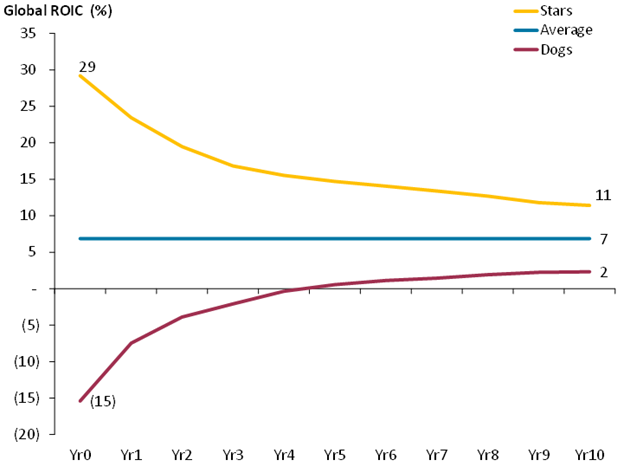
This means that very profitable firms decrease in profitability and low profitability firms increase in profitability. However, none of them reverts completely back to the mean. Therefore, the ValueModel opens the possibility to fade ROIC to a premium to WACC for very profitable firms and to a 20% discount to WACC for quite unprofitable firms. Fot average firms just choose “none”. Fading ROIC to WACC reflects the idea that firms can’t sustain excessive returns to infinity.

11. Growth (g) of cash flow at terminal period – The terminal growth rate is used to determine the value of a company within the terminal period. An estimate of terminal value is critical in financial modelling as it accounts for a large percentage of value. The terminal growth rate is the stable growth rate the firm can sustain in perpetuity and it can range between 0% and 5% in the ValueModel. The terminal growth rate should never exceed the growth rate of the economy. Theoretically, the stable growth rate could also be negative but this would mean that the analyst is assuming the firm to disappear over time. A simple proxy for the growth of the economy can be the risk-free rate.