How to Build a DCF Model: Step-by-Step Tutorial

A DCF model projects a company’s future cash flows, discounts them to today’s value, and produces an estimate of what the business is intrinsically worth. It is the core analytical tool in DCF valuation, the method used by investment banks, equity research analysts, and corporate finance teams to value companies based on fundamentals rather than market sentiment.

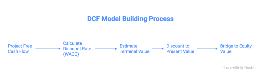
Building a reliable DCF model requires five steps: project free cash flows, calculate the discount rate, estimate terminal value, discount everything to present value, and bridge from enterprise value to equity value per share. Each step introduces assumptions that directly affect the output, so the quality of a DCF depends far more on judgment than on formula complexity.

This tutorial walks through each step with formulas, practical guidance, and the most common mistakes to avoid at each stage.

Step 1: Project Free Cash Flow

Free cash flow (FCF) is the foundation of every DCF; it represents the actual cash a company generates after funding operations and reinvesting in the business. You cannot build a DCF without first answering: how much cash will this business produce?

FCFF vs FCFE: Choose the Right Cash Flow

There are two variants, and the choice determines your entire model structure:

Free Cash Flow to the Firm (FCFF)

FCFF = EBIT × (1 – Tax Rate) + Depreciation & Amortization – Capital Expenditures – Change in Working Capital

FCFF measures cash available to all capital providers, both debt and equity holders. When you discount FCFF, you use WACC as the discount rate and arrive at enterprise value.

This is the most common approach in investment banking. It’s what Goldman Sachs used when valuing Twitter and what J.P. Morgan used in their Twitter fairness opinion.

Free Cash Flow to Equity (FCFE)

FCFE = Net Income + Depreciation & Amortization – Capital Expenditures – Change in Working Capital + Net Borrowing

FCFE measures cash available to equity holders only, after debt payments. Discount FCFE by the cost of equity to arrive at equity value directly.

Use FCFE when the company has a stable capital structure. Use FCFF when leverage is changing or when you want to separate operating performance from financing decisions. For a detailed comparison including the Dividend Discount Model, see our guide on which valuation method suits different company types.

How to Build the Revenue Forecast

The revenue forecast is the most important line in the model because everything else flows from it.

Do not just extrapolate historical growth rates. Instead, build revenue from its drivers:

• Volume × Price for product companies
• Users × Revenue per User for platform/tech companies
• Stores × Revenue per Store for retail
• Assets Under Management × Fee Rate for financial services

Our Coca-Cola revenue analysis demonstrates this approach: Coca-Cola’s revenue is driven by concentrates, not finished beverages, understanding that distinction completely changes your growth assumptions.

Forecasting period:

• 5 years for stable, mature businesses
• 7–10 years for high-growth companies that haven’t reached steady state
• The forecast should extend until the company reaches a sustainable, steady-state growth rate

Forecasting Expenses and Margins

After revenue, project operating expenses to arrive at EBIT:

• Use historical margins as a baseline, but adjust for known changes (new product launches, pricing pressure, scale effects)
• Be realistic, global data shows net profit margins average just 5.5% across all industries, yet analysts routinely project 15–20%. This is one of the most common valuation mistakes
• Consider margin trajectory: are margins expanding (scale/pricing power), stable, or compressing (competition/commoditization)?

Capital Expenditure and Working Capital

Two critical deductions from operating cash flow:

Capital expenditure (CapEx):

• Distinguish between growth capex and maintenance capex. Growth capex funds expansion; maintenance capex keeps existing assets running. Only maintenance capex is truly required.
• Understand the relationship between capex and depreciation. For a mature company, capex roughly equals depreciation. For a growing company, capex exceeds depreciation. If your model shows capex permanently below depreciation, the company is slowly liquidating its asset base.

Working capital changes:

• As revenue grows, working capital typically grows too (more receivables, more inventory)
• Model working capital as a percentage of revenue based on historical patterns
• Sudden swings in receivables collection or inventory conversion periods can significantly impact free cash flow

Step 2: Calculate the Discount Rate (WACC)

The discount rate reflects the opportunity cost and risk of the projected cash flows. For an enterprise DCF using FCFF, the correct discount rate is the weighted average cost of capital (WACC).

The WACC Formula

WACC = (E/V × Kₑ) + (D/V × Kd × (1 – T))

Component	What It Is	How to Find It
E/V	Equity weight	Market cap / (Market cap + Debt)
D/V	Debt weight	Debt / (Market cap + Debt)
Kₑ	Cost of equity	CAPM (see below)
Kd	Cost of debt	Interest expense / Total debt, or yield on traded bonds
T	Tax rate	Effective tax rate from financials

The weights should reflect the company’s target or optimal capital structure, not necessarily its current structure. See our analysis of optimal capital structure for why the distinction matters. And for a reality check on how theory maps to practice, read WACC: Theory Versus Reality.

Calculating Cost of Equity with CAPM

The Capital Asset Pricing Model (CAPM) is the standard:

Kₑ = Rf + β × (Rm – Rf)

Risk-free rate (Rf): Use the 10-year government bond yield of the country where the company primarily operates. The risk-free rate represents the return on a theoretically zero-risk investment. Current US rates are available from FRED.

Beta (β): Beta measures how much the stock moves relative to the market. A beta of 1.2 means the stock is 20% more volatile than the market.

Critical warning: do not use a raw calculated beta. Beta varies wildly depending on the time period, market index, and frequency you choose. A company can have a beta of 0.7 using 2-year weekly data and 1.4 using 5-year monthly data. Damodaran recommends using industry-average unlevered betas, then relevering for the company’s capital structure.

Equity risk premium (Rm – Rf): The equity risk premium is the extra return investors demand for owning stocks over risk-free bonds. It varies by country and market conditions. Damodaran publishes annually updated country equity risk premiums.

Quick sanity check: Damodaran publishes WACC by industry. If your calculated WACC is dramatically different from the industry average, double-check your inputs.

Step 3: Estimate Terminal Value

Terminal value captures the value of all cash flows beyond your explicit forecast period. It typically accounts for 60–80% of total enterprise value, making it the single most sensitive assumption in the model.

Method 1: Perpetuity Growth (Gordon Growth Model)

Terminal Value = FCFₙ × (1 + g) / (WACC – g)

Where:

• FCFₙ = free cash flow in the final projection year
• g = perpetual growth rate (typically 2–3%)
• WACC = discount rate

This method is a direct application of the Gordon Growth Model, originally developed for dividend valuation but equally applicable to free cash flows growing at a constant rate forever.

The golden rule: g should not exceed long-term nominal GDP growth (~2–3% for developed economies). A 4% perpetual growth rate implies the company will eventually become larger than the entire economy.

Method 2: Exit Multiple

Terminal Value = EBITDAₙ × Exit EV/EBITDA Multiple

This assumes the company could be sold at the end of the projection period at a market-comparable multiple. The exit multiple should reflect the company’s expected growth and return profile at steady state, not its current high-growth multiple.

Calibrating Terminal Value

The most important check: does the implied terminal multiple (from the perpetuity method) match what’s reasonable for the industry? And does the implied growth rate (from the exit multiple method) make sense?

Over time, return on invested capital should fade toward the cost of capital as competitive advantages erode. Our guide on ROIC fading and terminal multipliers explains how to align your terminal value with realistic long-term economics. Invested capital growth must also be consistent; you can’t project growth without the capital investment to fund it.

Step 4: Discount to Present Value

Now bring everything back to today’s dollars.

Enterprise Value = Σ (FCFₜ / (1 + WACC)ᵗ) + Terminal Value / (1 + WACC)ⁿ

This is a direct application of the present value concept, the foundation of the time value of money. Every future dollar is worth less today because of both the time delay and the risk involved.

Practical tips:

• Use mid-year convention (discount by t – 0.5 instead of t) if cash flows are generated throughout the year, not just at year-end
• Double-check that your discount periods are consistent. A common spreadsheet error is misaligning the first cash flow with the first discount period
• The terminal value gets discounted by the same number of periods as the last projected cash flow

Step 5: Bridge from Enterprise Value to Equity Value

The DCF gives you enterprise value, the total value of the business to all capital providers. To get to equity value (what the stock is worth), you need the equity bridge:

Equity Value = Enterprise Value – Net Debt – Minority Interest – Preferred Stock + Cash & Equivalents

Then:

Equity Value per Share = Equity Value / Fully Diluted Shares Outstanding

Item	What to Include
Net Debt	Total debt (short-term + long-term) minus cash
Minority Interest	Non-controlling interests in subsidiaries
Preferred Stock	Liquidation value of preferred equity
Cash	Cash and cash equivalents + short-term investments
Diluted Shares	Basic shares + in-the-money options (treasury stock method)

Compare the per-share intrinsic value to the current stock price:

• Intrinsic > Market Price → Stock is potentially undervalued
• Intrinsic < Market Price → Stock is potentially overvalued
• Intrinsic ≈ Market Price → Stock is fairly valued

For context on how this step fits into the broader stock valuation framework, see our overview of absolute vs. relative methods.

Sensitivity Analysis: Don’t Present a Point Estimate

A DCF produces a single number, but every input is an estimate. Always run sensitivity analysis on the three most impactful drivers:

Two-way sensitivity table (example):

	WACC 8%	WACC 9%	WACC 10%	WACC 11%	WACC 12%
g = 1.5%	$42	$36	$31	$27	$24
g = 2.0%	$46	$39	$33	$29	$25
g = 2.5%	$51	$42	$36	$31	$27
g = 3.0%	$57	$46	$39	$33	$29

Present your DCF as a valuation range (e.g., “$31–$46 per share”) rather than a single point estimate. This communicates analytical rigor and honest uncertainty.

Also stress-test:

• Revenue growth assumptions (±2–3%)
• Margin assumptions (±1–2% on EBIT margin)
• Terminal value as a % of total value (flag if >80%)

Common Mistakes at Each Step

Step	Mistake	Consequence
1. Cash Flows	Unrealistic margins	Inflated FCF → inflated valuation
1. Cash Flows	Ignoring the capex vs depreciation relationship	Understated reinvestment → overstated FCF
2. WACC	Using the calculated beta	Wrong cost of equity → wrong discount rate
2. WACC	Using book value weights instead of market value	Incorrect capital structure → incorrect WACC
3. Terminal	Growth rate > GDP growth	Implies company outgrows the economy
3. Terminal	Not checking the implied exit multiple	May imply unreasonable valuation
4. Discounting	Misaligning discount periods	Overstates or understates PV
5. Bridge	Forgetting the minority interest or preferred stock	Overstates equity value

For a comprehensive treatment, see Dr. Stotz’s complete guide to Damodaran’s valuation principles, which covers the mindset behind building reliable models.

DCF Model Checklist

Before presenting your DCF to anyone, verify:

• Revenue forecast built from drivers, not just growth rates
• Margins benchmarked against historical and industry averages
• CapEx consistent with growth assumptions and depreciation
• Working capital modeled as % of revenue
• WACC uses market-value weights
• Cost of equity uses industry-average beta (not raw calculated)
• Risk-free rate matches the company’s operating currency
• Terminal growth rate ≤ long-term GDP growth
• Terminal value < 80% of enterprise value (ideally 60–70%)
• Equity bridge includes all claims (debt, minorities, preferred)
• Diluted share count includes in-the-money options
• Sensitivity table on WACC and terminal growth rate
• Valuation presented as a range, not a point estimate

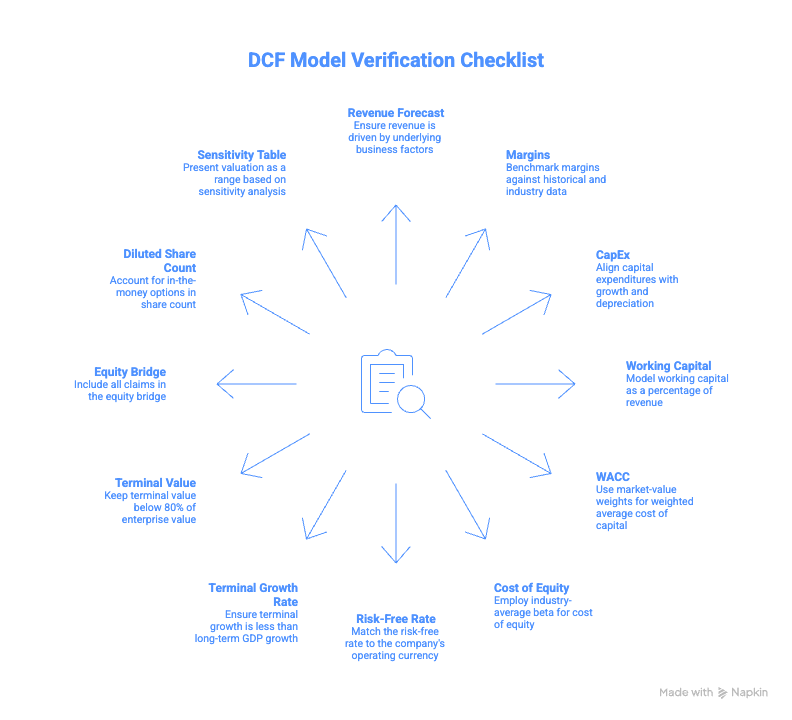
Frequently Asked Questions

What is the first step in building a DCF model?

Start by projecting the company’s free cash flows. You need to forecast revenue from its underlying drivers (volume, pricing, users), then project operating expenses, capital expenditures, and working capital changes. The quality of your cash flow projection determines the quality of the entire DCF.

Should I use FCFF or FCFE in my DCF?

Use FCFF (free cash flow to the firm) if the company’s leverage is changing or if you want to separate operating from financing performance; this is standard in investment banking. Use FCFE (free cash flow to equity) if the capital structure is stable and you want equity value directly. See our full comparison →

How do I calculate WACC for a DCF model?

WACC blends the cost of equity (via CAPM) with the after-tax cost of debt, weighted by the company’s market-value capital structure. Use industry-average betas and check your result against Damodaran’s WACC by industry data.

What perpetual growth rate should I use for the terminal value?

Use 2–3% for developed economies, aligned with long-term nominal GDP growth. Anything above 3% implies the company will eventually outgrow the economy. The Gordon Growth Model breaks down if g ≥ WACC, producing negative or infinite values.

How do I know if my DCF is reasonable?

Check three things: (1) Is the terminal value less than 80% of the enterprise value? (2) Does the implied exit multiple match comparable company multiples? (3) Does a sensitivity table produce a reasonable range? If the valuation swings wildly with small input changes, your assumptions need more work.

What data do I need to build a DCF model?

You need historical financial statements (from SEC EDGAR for US companies), a risk-free rate (from FRED), an equity risk premium (from Damodaran’s dataset), industry beta, and comparable company multiples for the exit multiple method.

Where can I practice building DCF models with real companies?

The Valuation Master Class Boot Camp teaches you to build DCF models on real companies over 12 weeks, producing 4 professional equity research reports with expert feedback from Dr. Andrew Stotz, a former #1-ranked equity analyst with 30+ years of experience.